A Closer Look at Linear Regression

Linear regression is often overlooked due to its simplicity and ubiquity. Let us remedy that.

Machine learning is fundamentally about learning functions. That is, for a set of $d$ input features predict some $d’$ output features. In other words, find a model $\hat{f} : \mathbb{R}^d \rightarrow \mathbb{R}^{d’}$ which approximates the true underlying function $f$ (assuming such a function exists). The space of functions $\mathbb{R}^d \rightarrow \mathbb{R}^{d’}$ is incredibly general, though, so we have to posit some good class of hypotheses, $\mathcal{F}$.

Linear regression chooses a simple but powerful class of hypotheses, the linear models:

\[\mathcal{F} = \{ x \mapsto W^T x : W \in \mathbb{R}^{d\times d'} \}\]

(note: you may be wondering where the intercept (or bias) term is. To accomplish this, we can either add an extra dimension to each data point with value 1, or we can fit a weight vector to $y - \bar{y}$). More simply put, consider a vector input features $(x_1,\ldots,x_d)$. For each target value $y_j$, we find coefficients $w_i$ such that

\[y_j \approx \hat{y}_j = w_1 x_1 + \ldots + w_d x_d\]

Let us further simplify the problem, and only consider single-target regression. Then our hypothesis class becomes

\[\mathcal{F} = \{ x \mapsto \beta^T x : \beta \in \mathbb{R}^d \}\]

Note: we switch to $\beta$ solely because it is more traditional for this restricted problem. So, we are trying to find $\beta$ such that we get good approximations for all $n$ data points (I will use the superscript in parentheses to denote indexing a specific variable, as opposed to the subscript, which I use for components of a vector):

\[\begin{align*} y^{(1)} \approx \hat{y}^{(1)} &= \beta_1 x_1^{(1)} + \ldots + \beta_d x_d^{(1)}\\ y^{(2)} \approx \hat{y}^{(2)} &= \beta_1 x_1^{(2)} + \ldots + \beta_d x_d^{(2)}\\ \ldots\\ y^{(n)} \approx \hat{y}^{(n)} &= \beta_1 x_1^{(n)} + \ldots + \beta_d x_d^{(n)}\\ \end{align*}\]

Now, I will assume that you both understand matrix multiplication and somehow have not seen linear regression (I acknowledge that is a somewhat small subset of people). The right hand sides of these equations are linear combinations of each data point, scaled by $\beta$. So, if we represent our data points $(x^{(1)}, \ldots, x^{(n)})$ as a matrix:

\[X = \begin{bmatrix} x^{(1)T}\\ x^{(2)T}\\ \ldots\\ x^{(n)T} \end{bmatrix}\]

Each element is actually a row vector of data, so we call the $n\times d$ matrix $X$ a data matrix. Then, we can represent our vector of targets $\hat{y}$ as the product $X\beta$. Expanding, we get:

\[y \approx \hat{y} = \begin{bmatrix} \hat{y}^{(1)}\\ \hat{y}^{(2)}\\ \ldots\\ \hat{y}^{(n)} \end{bmatrix} = \begin{bmatrix} X_{11}\beta_1 + \ldots + X_{1d}\beta_d\\ X_{21}\beta_1 + \ldots + X_{2d}\beta_d\\ \ldots\\ X_{n1}\beta_1 + \ldots + X_{nd}\beta_d \end{bmatrix} = X\beta\]

This is exactly the right hand side of the system of equations above!

Now we have a matrix representation of our solution. But what is this vector $\beta$? It combines features in such a way that the targets are approximated. We want a single number that is a measure of goodness of the approximation. A somewhat natural measure is the $l_2$ norm of the predictions, a generalization of Euclidean distance, denoted $||\bullet||_2$:

\[||z||_2 = \sqrt{z_1^2 + \ldots + z_d^2}\]

Square roots are nasty, so we usually work with the squared $l_2$ norm instead. Finding the coefficients is reduced to an optimization problem:

\[\beta_{OLS} = \underset{\beta}{\operatorname{argmin}}||X\beta - y||_2^2\]

Note that this is not the only solution for $\beta$. Specifically, this is the Ordinary Least Squares (OLS) formulation of linear regression.

The Cool Part

The most commonly used vector space is $\mathbb{R}^n$: n-dimensional vectors. It is important to realize that the study of vector spaces is more general than just that. Abstract vector spaces are general mathematical structures, representing things that can be multiplied by scalars and added together.

Consider the 2D projection problem. Suppose have a vector $v$ and a 1D subspace $U$ of $\mathbb{R}^2$ (i.e. a line), and we would like to find the closest element of $U$ to $v$.

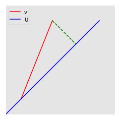
In this very concrete example, our geometric intuition tells us that the closest vector in $U$ to $v$ is that element $u$ such that an altitude can be dropped from the tip of $v$ to $u$. Clearly, any other line will have that same component $u$ plus some component in the perpendicular direction: it must be shortest. We call this the projection of $v$ onto $U$, and denote it $P_U v$. (aside: we can actually use linear algebra to quickly compute this: this image has $v = (2, 5)$, and $ U = \left\{ \left(\frac{1}{\sqrt{2}}, \frac{1}{\sqrt{2}}\right) a : a \in \mathbb{R} \right\} $. Because $e_1 = (\frac{1}{\sqrt{2}}, \frac{1}{\sqrt{2}})$ forms an orthonormal basis of $U$, we can use the formula $P_U v = \langle v, e_1 \rangle e_1 = (3.5, 3.5)$, the correct answer, noting that the inner product $\langle \bullet, \bullet \rangle$ is the dot product for $\mathbb{R}^n$).

What are we doing on this tangent? Well, recall that vector spaces are more general than $\mathbb{R}^n$. This suggests that the concept of projecting is more general than altitudes in planes. This turns out to be true, and projection can be used for lots of useful stuff (e.g. approximating nonlinear functions with polynomials: chapter 6 of Sheldon Axler’s Linear Algebra Done Right shows that on the interval $[-\pi, \pi]$, the function $\sin{x}$ is approximated extremely well by the polynomial $0.987862x - 0.155271x^3 + 0.00564312x^5$). Projection involves mapping a vector $v$ from a space $V$ to the closest vector on a subspace $U$ of $V$. Mathematically:

\[P_U v = \underset{u \in U}{\operatorname{argmin}} || v - u ||_2\]

We have $n$ $(x_i, y_i)$ pairs. The target vector $y$ is a subset of $\mathbb{R}^n$. Recall the range (column space) of $X$ is the space of linear combinations of its columns (denoting column $j$ of $X$ by $X_{*j}$:

\[\begin{align*} \text{range} X &= \left \{ \beta_1 X_{*1} + \ldots + \beta_d X_{*d} : \beta \in \mathbb{R}^d \right \}\\ &= \left \{ \beta_1 \begin{bmatrix} X_{11}\\\ldots\\X_{n1} \end{bmatrix} + \ldots + \beta_d \begin{bmatrix} X_{1d}\\\ldots\\X_{nd} \end{bmatrix} : \beta \in \mathbb{R}^d \right \} \end{align*}\]

The range of $X$ forms a subspace of $\mathbb{R}^n$, and $y \in \mathbb{R}^n$. That means that we can perform a projection of $y$ onto $\text{range} X$:

\[\begin{align*} P_{\text{range} X} y &= \underset{u \in \text{range} X}{\operatorname{min}} || y - u ||_2\\ &= \underset{\beta \in \mathbb{R}^d }{\operatorname{min}} ||y - X\beta||_2 \end{align*}\]

The optimal value, $\beta_{OLS} = \underset{\beta \in \mathbb{R}^d}{\operatorname{argmin}}|| X\beta - y ||$ is then related to $P_{\text{range} X}y$ by the following relation:

\[X\beta_{OLS} = \hat{y}\]

We would like to take the inverse of $X$ to compute $\beta$, but as $X \in \mathbb{R}^{n\times d}$, we must instead take the left psuedoinverse, $X^+$ (this gives us $X^+ X = I$, but not $X X^+ = I$):

\[\beta_{OLS} = X^+ \hat{y} = X^+ P_{\text{range} X} y\]

Let this sink in: approximating a target function on $n$ data points is the same thing as projecting the $n$ dimensional target vector onto the space of combinations of the feature columns. We are conceptually minimizing a distance between two vectors. This also gives us an interesting perspective of a function from target values to an optimal linear model, given the data $X$.

\[f_X : \mathbb{R}^n \rightarrow \mathbb{R}^d\]

We have brought the view of ordinary least squares from an optimization problem to a geometric interpretation. These intuitions are often much more valuable than knowing the algebra that goes into solving such a problem.