Coin Inference
There is a shocking disparity in the number of coins flipped by statisticians and laypeople. But, there is good reason for this. Coin flips are just about the simplest type of randomized experiment we can conduct. As such, there is much insight to gain from them.
Suppose we are interested in determining whether a coin is fair. More precisely, we are interested in the probability that some flip yields heads. It is common to refer to this value as $\theta$. Notice that this value is not random. A coin really has a singular, unchanging value for $\theta$. However, it is useful to think of the value as random, where the randomness comes from our lack of certainty in the actual value of $\theta$.
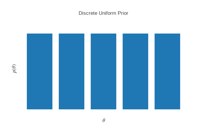
How would we determine $\theta$? Short of doing some intricate measurements of physical properties of the coin, all we can do is flip the coin. If the coin comes up heads, what can we conclude about $\theta$? Well, it’s a trick question. It depends on what values of $\theta$ we considered plausible before the flip; this is called the prior. Mathematically, we denote this $p(\theta)$. The prior is a function that maps from possible values to probabilities of those values. For coin flips, there is a common-sense restriction: because $\theta$ is a probability itself, it must be the case that $0 \leq \theta \leq 1$. Unfortunately, that’s all we get for free. Now, we’re thrust into the task of specifying exactly the form of the prior. There are an infinite number of possibile priors, and many could be plausible (a Buddhist might call this a thicket of views). For example, we might believe that $\theta$ can only take on the values 0, 0.25, 0.5, 0.75, or 1, and it could take any value with equal probability (each value takes on a probability of 1/5). We can visualize this graphically:
The workhorse of probabilistic inference is Bayes’ theorem; for us, it will take the following form:
\(\overbrace{p(\theta | \mathcal{D})}^{\text{Posterior}} = \frac{\overbrace{p(\mathcal{D} | \theta)}^{\text{Likelihood}} \overbrace{p(\theta)}^{\text{Prior}}} { \underbrace{p(\mathcal{D})}_{\text{Evidence}} }\).
We have already touched on the prior. The likelihood is a function that describes how likely we would be to observe some data $\mathcal{D}$, given the underlying distribution of the data, $\theta$. The denominator is a bit strange: how would we compute the probability of an observation? We have a likelihood function that tells us the probability of observing some data given the underlying parameter $\theta$, and the prior that tells us the probability that the true value of the parameter takes some value. We can combine this with the law of total probability:
\(\mathbb{P}[A] = \sum_{B_k}{\mathbb{P}[A \cap B_k]}\).
Here, ${B_k}$ is a set of disjoint events; that is, two distinct events $B_k$ and $B_j$ cannot co-occur (as a notational sidenote, I use $\mathbb{P}[\cdot]$ to denote a general probability fact, and $p(\cdot)$). Conveniently, the event of that a parameter takes one value is disjoint from the event that it takes another (e.g. $\mathbb{P}[\theta = 0.25 \cap \theta = 0.75] = 0$). Then, we can decompose the evidence:
\(p(\mathcal{D}) = \sum_{\theta'}{p(\mathcal{D} \cap \theta')} = \sum_{\theta'}{p(\theta') p(\mathcal{D} | \theta')}\).
Plugging in each of these terms to Bayes’ theorem gives us the posterior distribution. This is exactly what we are looking for: we have some prior beliefs about the value of $\theta$, and we then make observations. For example, I flipped a coin 10 times and observed the following: T, T, H, H, H, T, H, T, H, T.
How do we update our information after the first flip? First, we need to know how to compute likelihood. Remember, $\theta$ is the probability of getting heads. Then, $p(\mathcal{D}=H | \theta) = \theta$, and similarly, $p(\mathcal{D}=T | \theta) = 1 - p(\mathcal{D}=H | \theta) = 1 - \theta$. We can write the probability of a sequence of $N$ flips compactly: $p(\mathcal{D} | \theta) = \theta^{n} (1 - \theta)^{N - n}$ where $n$ is the number of observed heads.
Let us compute the posterior after the first flip:
\[\begin{align*} p(\theta | \mathcal{D} = T) &= \frac{p(\mathcal{D} = T | \theta) p(\theta)}{p(\mathcal{D} = T)}\\ &= \frac{(1 - \theta)(0.2)}{\sum_{\theta' \in \{0, 0.25, 0.5, 0.75, 1\}}{0.2(1 - \theta')}}\\ \end{align*}\]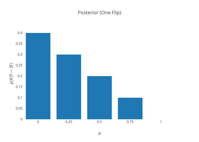
These results make sense: we saw a tail, so it is now impossible that the probability of getting a head is 100%. Similarly, the probabilities for lower values of $\theta$ increased. Now, the most likely value is 0.
We can iterate this process for the entire dataset. After the ten flips, it looks like this:
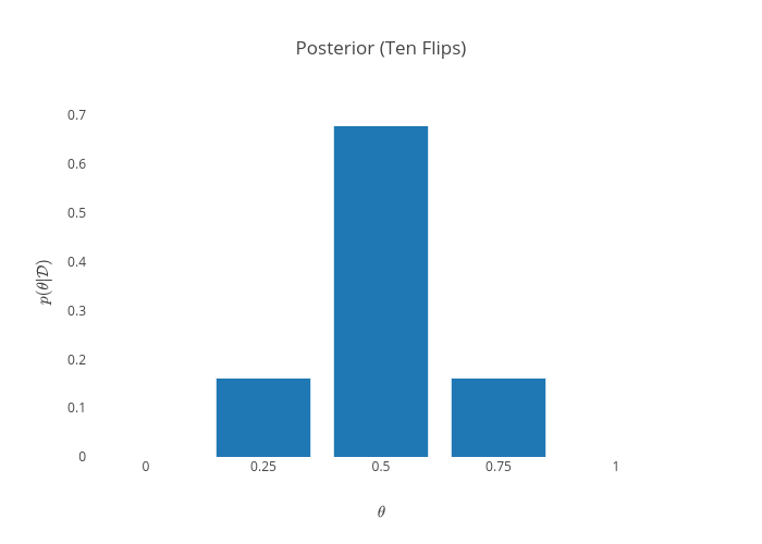
Note that this was a particularly lucky sequence of coin tosses - exactly half of the flips were heads. An unlucky sequence of tosses (one that seems to indicate a lower value of $\theta$) is entirely possible. Suppose we got instead 10 tails in a row. That would yield the following posterior:
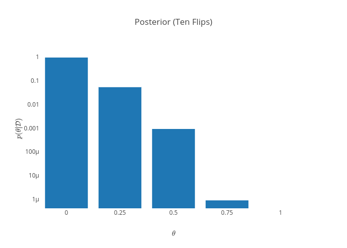
This indicates near-certainty that the coin is two-sided tails. Still, it does not discount the possibility that the coin could still be fair. After all, the probability of getting 10 tails in a row with a fair coin is $\frac{1}{2^{10}} = \frac{1}{1024}$. Unlikely, but entirely possible. That is an advantage of probabilistic modelling - low-probability events are still kept around.
Continuous Inference
So far, we have only explored inference using a discrete uniform prior with five elements. Though it is simple to think about, we are disallowing for the possibility of a value of $\theta$ not in that tiny subset of values. This could be sufficient in some situations, but it would be nice to have more flexibility. We could fill in some of the gaps - what if we included 50 values, uniformly distributed? That prior would look like this:
\[p(\theta) = \begin{cases} 1 / 50 & \theta \in \{0/50, 1/50,\ldots,50/50\}\\ 0 & \text{otherwise} \end{cases}\]What if we did 100? 1000? It might be tough to keep track of all those possibilities. Could we take this process to the limit?
It turns out, we can. This yields the continuous uniform distribution, denoted $\operatorname{unif}(a, b)$, where $a$ and $b$ are the bounds. There’s a problem in defining the probability for this; there are an infinite number of values in any non-empty real interval. That would indicate that the probability becomes 0 in the limit. So it seems we’ve reached a paradox; the true value of $\theta$ must be somewhere in the interval $[0,1]$, but the probability of it being in any one location is zero.
Picture holding a bowling ball. It’s heavy. It obviously has some mass. Yet imagine the mass some small part of the ball - it weighs less than the bowling ball. Consider the limit of zooming in on some infinitely small point on the ball. It has zero mass. We’re facing the same paradox, but there is another useful concept here: density. Though the mass goes to zero as we focus in, the density goes to some nonzero value.
Someone had the clever idea of introducing an analogous idea for probability distributions. Previously, we were dealing with probability mass functions: the “mass” of the distribution is centered around a few discrete values. For continuous distributions, we consider probability density functions. It is true, no individual point has any probability “mass”, but it does have a probability “density”. We can get back to a mass by considering a region of the space of inputs, and integrating over it.
The continuous uniform distribution on the interval $[0,1]$ has a probability density function (pdf) of the following form:
\[p(x) = 1\]To extract probabilities over a certain range $[a,b]$, we integrate over the pdf in that range:
\[p(a \leq x \leq b) = \int_a^b{p(x')dx'}\]What’s really cool about this switch to continuous inference is that it just works (TM). Given some data $D$ and a prior $p(x)$ over the data, the posteror distribution is defined exactly as it was before:
\[p(x|D) = \frac{p(D|x)p(x)}{p(D)}\]One caveat: the denominator here is an integral that can be really painful to compute for any practical problem - have you ever done a double integral? A triple integral? Well, the denominator will have an integral for every variable. In practice, this term is not computed in an exact form. There are two common ways to do this:
- Markov Chain Monte Carlo (MCMC): this technique involves sampling from the posterior distribution using techniques that avoid having to compute the denominator. The important trick here is that if you computing the ratio of densities: \(\frac{p(x|D)}{p(y|D)} = \frac{p(D|x)p(x)}{p(D|y)p(y)}\)
- Variational Inference (VI): this involves approximating the posterior distribution by using a family of approximate functions, and using gradient descent to optimize its similarity to the true posterior, using a ‘metric’ of similarity called KL Divergence
I’m a little sick of writing plotting code now, so I’m just gonna leave that as an exercise to the reader.