Compiling Lambda Calculus Programs
I’ve been working on a lambda calculus interpreter for a while. One of the many reasons it is unpleasant to program in lambda calculus is that every time you want to use a function, you have to redefine it in place. The simple extension I wanted to add was declarations, so we can, for example, say $T = \lambda t f.t$ once, and then refer to $\lambda t f.t$ by the identifier $T$. For notational convenience, let $\langle Ident\rangle$ denote the binding corresponding to $Ident$, and $Ident_C$ denote the compiled version of $Ident$. Then, suppose we have another definition $or = \lambda p ~q.p ~T ~q$. This definition can be expanded by substituting $T$ in the definition of $or$, i.e. $or’ = (\lambda p ~q.p ~T ~q)[T/\lambda t ~f.t]$. The obvious way to express that we want to perform this substitution is with an abstraction: \(or_C = (\lambda T.\langle or\rangle)\langle T\rangle\)
We can inject any number of dependencies in this manner. Given a declaration $X$, and assuming every free variable $\tau\in \operatorname{FV}(\langle X\rangle)$ is a dependency, collect each dependency $\tau_1,\ldots,\tau_n$ of $\langle X\rangle X$. Then, our compiled declaration is \(X_C = (\lambda \tau_1\ldots \tau_n.\langle X\rangle)\langle \tau_1\rangle \ldots \langle \tau_n \rangle.\)
Let’s do something more complicated. Consider the following bindings: \(T = \lambda t ~f.t\\ F = \lambda t ~f.f\\ or = \lambda p~q.p ~T ~q\\ and = \lambda p~q.p ~q ~F\\ not = \lambda p.p ~F ~T\\ xor = \lambda p~q.and ~(or ~p ~q) ~(not ~(and ~p ~q))\)
How do we get $xor_C$? We need to be careful about the order in which we substitute, so that the substituted dependencies are the fully compiled versions (i.e. they do not have free variables). We can visualize these dependencies as a graph:

Here we have an arrow $x\rightarrow y$ if $y$ appears as a direct dependency of $x$. Before we compile $xor$, we must compile its dependencies $or$, $and$ and $not$. Notice that these dependencies do not depend on each other, and so it does not matter the order we compile these three relative to each other. One such compilation order that would work is \([T,F,or,and,not,xor]\)
We want an ordering such that if there is a dependency path from $x$ to $y$ ($x$ depends on $y$ directly or indirectly), then $y$ appears before $x$ in the ordering. This is almost the definition of a topological sort, but the arrows in the dependency graph $G$ are in the wrong direction. There are two easy ways to address this. Either we reverse the topological sort of $G$, or we use the topological sort of the reverse graph $G^R$.
To recap, our algorithm so far is the following. Compute the dependencies (free variables) of each binding $\tau_i = E_i$ (call them $D_i$). Then, construct the dependency graph $G$ with a node for each identifier, such that there is an edge between $\tau_i$ and $\tau_j$ when $\tau_j \in D_i$. Now, compute a topological sort of $G$ and reverse it: call this $S$. For each identifier $\tau_i \in S$ (in order), let $D_i = {\sigma_1,\ldots,\sigma_n}$, and construct the compiled binding \({\tau_i}_C = (\lambda \sigma_1\ldots\sigma_n.\langle \tau_i\rangle)\langle{\sigma_1}_C\rangle\ldots\langle{\sigma_n}_C\rangle.\)
This is possible because we know we have compiled $\sigma_j$ previously. Finally, replace each binding with its compiled version. In other words, create new bindings $\tau_i = \langle {\tau_i}_C \rangle$.
You might have noticed something. Topological sorts can only be defined for directed acyclic graphs - if $G$ had a cycle between $u$ and $v$, it would be impossible to construct an ordering such that $u$ appears before $v$ and vice versa. This is not some esoteric use case; in a dependency graph, such a cycle would occur in the case of recursive functions and mutually recursive functions (a function can depend on itself, so $G$ can have self-cycles). We will deal with the former case first.
Because pure untyped lambda calculus has no notion of bindings, a function cannot refer to itself by name - the trick is to bundle a the function in it’s own call. To accomplish this, we need a combinator $Fix$ such that \(Fix ~f =_{\beta} f ~(Fix ~f).\)
Our choice of fix point combinator depends on the choice reduction strategy. For normal order evaluation, we use the $Y$ combinator: \(Y = \lambda g.(\lambda x.g ~(x ~x))(\lambda x.g ~(x ~x)).\)
As an aside, we can use the $Z$ combinator for applicative order evaluation, where $Z = \lambda g.(\lambda x.f ~(\lambda v.x ~x ~v)) (\lambda x.f~(\lambda v.x~x~v))$ - the $v$ abstractions prevent the fix point from expanding too much. To take advantage of this, we define our recursive function as a function that takes itself as an argument. The classic example is the factorial function, defined as \(n! = \begin{cases}1 & n = 0\\n \times (n - 1)! & otherwise\end{cases}\)
In the expanded syntax, we can say \(Fact ~n = (equal ~n ~0) ~1 ~(mult ~n ~(Fact ~(pred ~n))).\)
Because $Fact$ appears free in its own definition, it has a dependence on itself. It is simple to expand our algorithm to take care of recursive functions. We still use the same topological sort of the identifiers; for each identifier $\tau$ with a self-dependence, we perform an additional step. Let ${\sigma_1,\ldots,\sigma_n} = FV(\langle \tau\rangle)$. Then, $\tau$ has the following compiled form:
\[\tau_C = Y ~[(\lambda ~\sigma_1\ldots~\sigma_n~\tau.\langle\tau\rangle)~\sigma_1\ldots~\sigma_n].\]Mutually recursive functions are a good deal more complicated, because they ruin the acyclic structure of the program. However, just because our list of bindings has some mutually recursive functions doesn’t mean that the whole graph is fundamentally acyclic. We can identify the mutually recursive functions in $G$ as the strongly connected components of $G$. Split $G$ into the components $G_1,\ldots,G_m$, representing the groups of mutually recursive functions, and let $G_C$ represent the condensation of $G$ - that is, an acyclic summary of $G$ in which each node represents a strongly connected component of $G$. Instead of compiling each binding separately, we consider each strongly connected component.
Notice that each component $\tau_i$ in a strongly connected component $G_l$ needs to know the definition of each other component, because even if $\tau_i$ doesn’t use some other $\tau_j \in G_l$, $\tau_i$ indirectly depends on $\tau_j$. In a simply recursive function, the function only needs to have itself passed as a parameter - we generalize this to multiple functions by “bundling” the definition of each function in the strongly connected component, and passing this bundle $B$ to the recursive function. We then can refer to each function by selecting the right component. Suppose $G_l$ has bindings $\tau_1,\ldots,\tau_k$. Define the selector function $s_i = \lambda \tau_1\ldots\tau_k.\tau_i$ - $s_i$ selects the $i$-th component from the bundle. Then, let
\[\tau_i' = [\lambda \sigma_1\ldots\sigma_p ~b.(\lambda \tau_1\ldots\tau_k.\langle \tau_i\rangle) ~(b ~\langle s_1\rangle)\ldots(b ~\langle s_k\rangle)]\langle \sigma_1\rangle\ldots\langle\sigma_1\rangle\]Then we define the bundle as follows:
\(\beta = \lambda b ~s.s ~\langle\tau_1'\rangle\ldots\langle\tau_k'\rangle ~b\) \(B = Y \beta\)
Then, our compiled terms are as follows: \({\tau_i}_C = B ~s_i\)
As an example, consider the (terrible) algorithm for computing whether a number is odd or even: \(odd = \lambda n.(isZero ~n) ~F ~(even ~(pred ~n))\\ even = \lambda n.(isZero ~n) ~T ~(odd ~(pred ~n))\)
Let’s compute the intermediate terms: \(odd' = \lambda b ~n.((\lambda odd ~even.(isZero ~n) ~F ~(even ~(pred ~n))) ~(b ~s_1) ~(b ~s_2))\\ even' = \lambda b ~n.((\lambda odd ~even.(isZero ~n) ~T ~(odd ~(pred ~n))) ~(b ~s_1) ~(b ~s_2))\)
Then, the bundle is \(\beta = \lambda b ~s.s \langle odd'\rangle \langle even'\rangle ~b\\ B = Y \beta.\)
The final compiled terms are as follows: \(odd_C = B ~s_1\\ even_C = B ~s_2\)
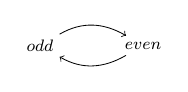
As an example, let’s determine if 2 is even:
\[\begin{align} even ~2 &= Y ~\beta ~s_2 ~2\\ &= \beta ~B ~s_2 ~2\\ &= s_2 ~odd' ~even' ~B ~2\\ &= even' ~B ~2\\ &= ((\lambda odd ~even.(isZero ~2) ~T ~(odd ~(pred ~2))) ~(B ~s_1) ~(B ~s_2))\\ &= (isZero ~2) ~T ~(B ~s_1 ~(pred ~2))\\ &= B ~s_1 ~(pred ~2)\\ &= \beta B ~s_1 ~(pred ~2)\\ &= s_1 ~odd' ~even' ~B ~(pred ~2)\\ &= odd' ~B ~(pred ~2)\\ &= ((\lambda odd ~even.(isZero ~(pred ~2)) ~F ~(even ~(pred ~(pred ~2)))) ~(B ~s_1) ~(B ~s_2))\\ &= (isZero ~(pred ~2)) ~F ~(B ~s_2 ~(pred ~(pred ~2)))\\ &= B ~s_2 ~(pred ~(pred ~2))\\ &= \beta ~B ~s_2 ~(pred ~(pred ~2))\\ &= s_2 ~odd' ~even' ~B ~(pred ~(pred ~2))\\ &= even' ~B ~(pred ~(pred ~2))\\ &= ((\lambda odd ~even.(isZero ~(pred ~(pred ~2))) ~T ~(odd ~(pred ~(pred ~(pred ~2))))) ~(B ~s_1) ~(B ~s_2))\\ &= (isZero ~(pred ~(pred ~2))) ~T ~(B ~s_1 ~(pred ~(pred ~(pred ~2))))\\ &= (isZero ~0) ~T ~(B ~s_1 ~(pred ~(pred ~(pred ~2))))\\ &= T \end{align}\]From a dependency standpoint, we have transformed the graph from this (ignoring non-recursive dependencies):
to this:
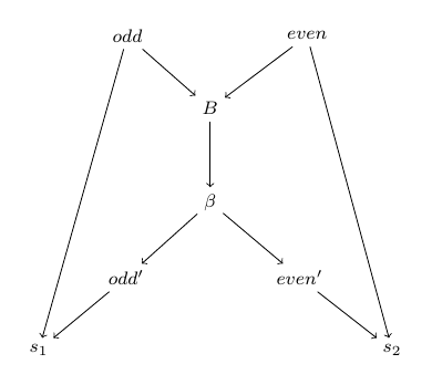
Notice that we have transformed the strongly connected component into an acyclic subgraph. We can perform this step on each strongly connected component and transform the original cyclic graph $G$ into an acyclic equivalent $G’$. Specifically, for each strongly connected component with bindings $\tau_1,\ldots,\tau_n$, collect acyclic equivalent with terms $\tau_i$, $\tau’_i$, $s_i$, $B$, and $\beta$. We can regard the $\tau_i$ as the recursive interface to the function, while the $\tau’_i$ are the implementations of the non-recursive kernel of the original cyclic implementation. As such, the dependencies of the cyclic $\tau_i$ are now dependencies of the $\tau’_i$, while the (non-cyclic) dependees of the cyclic $\tau_i$ (that is, nodes $v$ such that there is an edge $(v,\tau_i)$ in $G$) become dependees of the acyclic $\tau_i$. Because $G’$ is a DAG, we can obtain a topological sort, so we can simply apply the previous algorithm to $G’$ to obtain our compiled terms.
We can define $odd$ and $even$ explicitly in Haskell (note that $\texttt{fix}$ is a fix point combinator in Haskell):
import Data.Function (fix)

data Fun = Odd | Even deriving (Eq)
data Description = Desc { action :: Fun, input :: Int } deriving (Eq)
type Result = Either Bool Description

even', odd' :: Int -> Result
even' n = if n == 0
            then Left True
            else Right (Desc Odd (n - 1))
odd' n = if n == 0
            then Left False
            else Right (Desc Even (n - 1))

dispatch :: Description -> Result
dispatch (Desc f n) = case f of
    Odd -> odd' n
    Even -> even' n

bundle :: Result -> Bool
bundle = fix (\bundle' result -> case result of
                Left p -> p
                Right desc -> bundle' desc)

even, odd :: Int -> Bool
even n = bundle (Right (Desc Even n))
odd n = bundle (Right (Desc Odd n))
This is, of course, an awful way to compute parity of a number. Regardless, I think it’s interesting that it’s possible to factor out even mutual recursion. Here’s a way to interpret what’s going on here: $\texttt{even’}$ and $\texttt{odd’}$ compute either a final value or a description of what computation should happen next, without actually performing that computation. Given this description, we can get an actual computation, through the $\texttt{dispatch}$ function. However, these two functions still don’t perform the whole computation. We need to chain these computations together recursively. The $\texttt{bundle}$ function takes a result and decides whether to terminate or recurse based on its value. Finally, to get the original interface of the even and odd functions, we feed a description of the initial computations we want to perform into $\texttt{bundle}$.